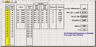
As with any hypothesis test, the output states whether to reject or not reject the Null Hypothesis and the specified alpha level. In this case, the Null Hypothesis states that the data sample came from a normally distributed population. This Null Hypothesis is rejected only if Test Statistic W is less than the critical value of W for a given alpha level and sample size.
Overview of the Shapiro-Wilk Test For Normality
The Shapiro-Wilk Test is a hypothesis test that is widely used to determine whether a data sample is normally distributed. A test statistic W is calculated. If this test statistic is less than a critical value of W for a given level of significance (alpha) and sample size, the Null Hypothesis which states that the sample comes from a normally distributed population is rejected. Keep in mind that passing a hypothesis test for normality only allows one to state that no significant departure from normality was found.The Shapiro-Wilk Test is a robust normality test and is widely-used because of its slightly superior performance against other normality tests, especially with small sample sizes. Superior performance means that it correctly rejects the Null Hypothesis that the data are not normally distributed a slightly higher percentage of times than most other normality tests, particularly at small sample sizes.
The Shapiro-Wilk normality test is generally regarded as being slightly more powerful than the Anderson-Darling normality test, which in turn is regarded as being slightly more powerful than the Kolmogorov-Smirnov normality test. The Shapiro-Wilk normality test is affected by tied data values but less so than the Anderson-Darling normality test.
An abbreviated description of the steps of the Shapiro-Wilk normality test is as follows:
- Sort the raw data in an ascending sort
- Arrange the sorted data into pairs of successive highest and lowest data values
- Calculate the difference between the high and low value of each pair
- Multiply each difference by an “a Value” from a lookup table
- Calculate test statistic W
- Compare test statistic W with a W Critical Value obtained from a lookup table
- Reject the Null Hypothesis stating normality only if W is smaller than W Critical

(Click On Image To See a Larger Version)
Step 1 – Sort Data in an Ascending Sort
Enter the Raw Data and Alpha Level
First, paste in the raw, unsorted data and set the alpha level in the yellow cells as follows:
(Click On Image To See a Larger Version)
This Shapiro-Wilk normality test in Excel has the capability to handle up to 20 data points. This data sample contains only 15 data points but the Excel worksheet below indicates the capability for an additional 5 data points in the empty yellow cells. Expanding the capability of this Excel test to handle a larger number of data points would be a straightforward matter of making adjustments to the Excel formulas.
The alpha level should be set at 0.01, 0.05, or 0.10 because critical values of W are provided here only for those common alpha levels. If alpha is set at a different level, the following warning appears as a result of the If-Then-Else statement seen in the previous image:

(Click On Image To See a Larger Version)
Sort the Raw Data Using Formulas, Not the Excel Sorting Tool
The most efficient way to sort data is with the use of formulas as shown. The Excel sorting tool must be manually re-run whenever the raw data is changed in any way. The following formula will automatically resort the data if any data are changed or added. The following formulas produce an ascending sort. To create a descending sort, simply swap the word LARGE for SMALL within the formula.
(Click On Image To See a Larger Version)
Step 2 – Obtain “a Values” From the “a Value Lookup Table”
The Table of a Values
The a Values are constants that are calculated from the means, variances, and covariances of the order statistics of a sample of size n from a normal distribution. The a Value table is shown as follows for data samples varying in size from n = 2 up to n = 50.
(Click On Image To See a Larger Version)

(Click On Image To See a Larger Version)

(Click On Image To See a Larger Version)

(Click On Image To See a Larger Version)

(Click On Image To See a Larger Version)
Create Labels for the a Values
The first step in obtaining the correct a Values is to create the proper number of labels for the a Values.The number of a Values needed depends on the sample size n. If n is an even number, the number of a Values equals n / 2. If n is an odd number, the number of a Values equals (n-1) / 2. This can be implemented with the following formulas:

(Click On Image To See a Larger Version)
Lookup a Values on the a Value Lookup Table
The a Values can now be looked up on the a Value table previously shown. An Index formula is a straightforward way implementing this. The Excel Index function is its simplest form has the following format:Index(array, row number, column number) and returns the data value located in the specified row and column of the given array. The row and column number are relative to the cell in the upper-left corner of the array. Note that the array containing the a Values starts in cell H58 at the upper left corner and finishes in cell BE82 in the lower right corner.

(Click On Image To See a Larger Version)
Step 3 – Pair Up Successive Highest-Lowest Data Values
Create X Labels for Data Sample Values
Each sorted data sample value will have an X Label. This is implemented with the following formulas:
(Click On Image To See a Larger Version)
The following is a close-up of the formulas to create the labels for the X Values:

(Click On Image To See a Larger Version)
The X Values are then obtained using the following formulas:

(Click On Image To See a Larger Version)
Create the Upper Value of Each Data Pair
The labels for the upper X Values of each data pair are created as follows: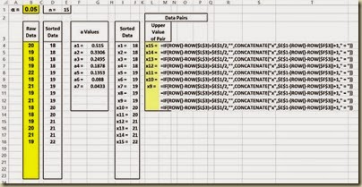 The following is a close-up of the formulas to create the labels for the upper X Values:
(Click On Image To See a Larger Version)
The upper X Values of each data pair are the obtained using the following set of formulas:

(Click On Image To See a Larger Version)
Here is a close-up of those formulas:
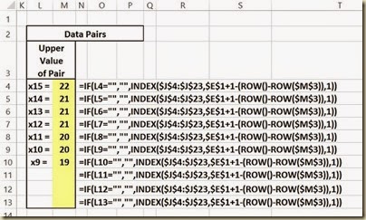
(Click On Image To See a Larger Version)
Create the Lower Value of Each Data Pair
The labels for the lower X Values of each data pair are created as follows: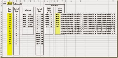
(Click On Image To See a Larger Version)
The following is a close-up of the formulas to create the labels for the lower X Values:

(Click On Image To See a Larger Version)
The lower X Values of each data pair are the obtained using the following set of formulas:

(Click On Image To See a Larger Version)
Here is a close-up of those formulas:

(Click On Image To See a Larger Version)
Step 4 – Calculate the Difference Within Each Pair
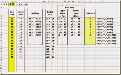
(Click On Image To See a Larger Version)
Here is a close-up of the difference formulas:

(Click On Image To See a Larger Version)
Step 5 – Calculate a * Difference

(Click On Image To See a Larger Version)
Here is a close-up of those formulas:

(Click On Image To See a Larger Version)
Step 6 – Calculate b, SS, and Test Statistic W
b equals the sums of the product of a * pair difference.SS is the sum of the squared deviations of x from the mean x. Excel formula DEVSQ() performs this.
Test Statistic W equals b2/SS.

(Click On Image To See a Larger Version)
Here is a close-up of these formulas:

(Click On Image To See a Larger Version)
Step 7 – Lookup W Critical Values
Each unique combination of sample size and alpha level has its own critical W value. The following is a table of the respective critical W value for each combination of n and alpha up to a sample size of 50 and 3 common levels of alpha.
(Click On Image To See a Larger Version)

(Click On Image To See a Larger Version)

(Click On Image To See a Larger Version)
Here is a close-up of the formulas. The If-Then-Else statement that looks up the critical W value is the following:
=IF(OR(B1=0.01,B1=0.05,B1=0.1),INDEX(BL18:BN67,U14,IF(U12=0.01,1,IF(U12=0.05,2,IF(U12=0.1,3)))),”alpha must be set to 0.01, 0.05, or 0.10”)
The INDEX() function looks up the critical W values in the array starting in cell BL18 in the upper left corner and ending in cell BN67 in the lower right corner.

(Click On Image To See a Larger Version)
Step 8 – Determine Whether or Not To Reject Null Hypothesis By Comparing W to W Critical
The Null Hypothesis is rejected only if Test Statistic W is smaller the critical W value for the given sample size and alpha level. The Null Hypothesis states that the sample came from a normally distributed population. The Null Hypothesis is never accepted but only rejected or not rejected. Not rejecting the Null Hypothesis does not automatically imply that the population from which the sample was taken is normally distributed. This merely indicates that there is not even evidence to state that the population is likely not normally distributed for the given alpha level. As with all hypothesis tests, alpha = 1 - level of certainty. If a 95-percent level of certainty is required to reject the Null Hypothesis, the alpha level will be 0.05.
(Click On Image To See a Larger Version)
Here is a close-up of the formulas to compare W with W Critical:

(Click On Image To See a Larger Version)
The complete Shapiro-Wilk test of normality appears in Excel as follows:
(Click On Image To See a Larger Version)
Excel Master Series Blog Directory
You Will Become an Excel Statistical Master!
MONDAY, APRIL 13, 2015
Simplifying Excel Ranking Functions: RANK(), RANK.AVG(), RANK.EQ(), PERCENTILE(), PERCENTILE.INC(), PERCENTILE.EXC(), QUARTILE(), QUARTILE.INC(), QUARTILE.EXC()
Simplifying Excel Ranking
Functions: RANK(),
RANK.AVG(), RANK.EQ(),
PERCENTILE(),
PERCENTILE.INC(),
PERCENTILE.EXC(),
QUARTILE(), QUARTILE.INC
(), QUARTILE.EXC()
Simplifying RANK(), RANK.EQ(), and RANK.AVG()
Ranking functions RANK(), RANK.EQ(), and RANK.AVG() return the rank of a data value within a data set. Prior to Excel 2010 RANK() was the sole ranking function. In Excel 2010 and beyond RANK() will still work but its functionality has been duplicated by a new ranking function RANK.EQ(). In addition, another useful ranking function RANK.AVG() has been added.The format of each of these functions is as follows:
RANK(value to be ranked, data range, [order])
RANK.EQ(value to be ranked, data range, [order])
RANK.AVG(value to be ranked, data range, [order])
The value to be ranked is a specific number or value is a data set that will be ranked. The data range represents the set of values that will provide the basis for the ranking. The order is an optional value. Setting the order to 0 or leaving it blank will rank data in descending order, i.e., the highest value in the data range will be assigned a rank = 1. Setting the order to 1 will rank data in ascending order, i.e., the lowest value in the data range will be assigned a rank = 1.
The difference between RANK.EQ() and RANK.AVG() is how tied data values within the data set are ranked. RANK.EQ() assigns the lowest rank of the tied values to all of the tied values. RANK.AVG() assigns the average rank of the tied values to all of the tied values.
RANK.AVG() is useful when performing certain nonparametric tests in Excel. Several nonparametric tests require that data be ranked with tied data values being assigned the average rank of the tied values as is done by RANK.AVG(). These nonparametric tests include the Mann-Whitney U Test, the Wilcoxon Signed-Rank Test, and the Friedman Test.
The functionality of the RANK() function is shown as follows. The raw data that is being ranked has already been sorted in order to more easily convey the functionality of the RANK() function.

(Click On Image To See a Larger Version)
The functionality of the RANK.EQ() function is shown in the following diagram. RANK.EQ() is equivalent to RANK() and should now be used in its place. Note that tied data values are all assigned the lowest rank of the tied values. The raw data that is being ranked has already been sorted in order to more easily convey the functionality of the RANK.EQ() function.

(Click On Image To See a Larger Version)
The functionality of the RANK.AVG() function is shown in the following diagram. Note that tied data values are all assigned the average rank of the tied values. There is no equivalent to this function in versions of Excel prior to 2010. The raw data that is being ranked has already been sorted in order to more easily convey the functionality of the RANK.AVG() function.

(Click On Image To See a Larger Version)
Simplifying PERCENTILE(), PERCENTILE.INC(), and PERCENTILE.EXC()
Percentile functions PERCENTILE(), PERCENTILE.INC(), and PERCENTILE.EXC() return the value at a given percentile in relation to a given data set. For example, given the data set {1, 3, 5, 13, 15} in cells A2:A6, PERCENTILE(A2:A6,0.3) = 3.4. This means that the value 3.4 occupies the 30th percentile of the given data set.An example of the use of the percentile functions would be to determine which test scores within a group of test score are at or above the 95th percentile of the group. The percentile functions would return that value that would occupy that 95th percentile of the group.
The percentile functions are typically used to establish a threshold of acceptance or failure.
Prior to Excel 2010 PERCENTILE() was the sole percentile function. In Excel 2010 and beyond PERCENTILE() will still work but its functionality has been duplicated by a new percentile function PERCENTILE.INC(). In addition, another percentile function PERCENTILE.EXC() has been added.
The format of each of these functions is as follows:
PERCENTILE(data range, percentile)
PERCENTILE.INC(data range, percentile)
PERCENTILE.EXC(data range, percentile)
The percentile can be any number between 0 and 1.
The value to be ranked is a specific number or value is a data set that will be ranked. The data range represents the set of values that will provide the basis for the ranking. The order is an optional value. Setting the order to 0 or leaving it blank will rank data in descending order, i.e., the highest value in the data range will be assigned a rank = 1. Setting the order to 1 will rank data in ascending order, i.e., the lowest value in the data range will be assigned a rank = 1.
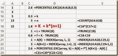
Both PERCENTILE.EXC() and PERCENTILE.INC() and its equivalent PERCENTILE() first rank the values in the given data set from 1 (assigned to the lowest value in the data set) to n (assigned to the highest value in the data set). The rank K is then calculated. The main difference between is the method of calculating K as shown in the following Excel algorithms for these functions. If K is not an integer value, linear interpolation between the nearest values in the data set to determine the value that would occupy the given percentile.
Another difference between the percentile functions is that PERCENTILE.EXC only works if k is between 1/n and 1-1/n, where n is the number of elements in array. PERCENTILE.INC works for any value of k between 0 and 1.
The Excel algorithm for equivalent functions PERCENTILE() and the equivalent PERCENTILE.INC() is as follows:

(Click On Image To See a Larger Version)
The Excel algorithm for PERCENTILE.EXC() is as follows:
(Click On Image To See a Larger Version)
Simplifying PERCENTRANK(), PERCENTRANK.INC(), and PERCENTRANK.EXC()
PERCENTRANK(), PERCENTRANK.INC(), and PERCENTRANK.EXC() are the inverse functions of PERCENTILE(), PERCENTILE.INC(), and PERCENTILE.EXC().PERCENTRANK(), PERCENTRANK.INC(), and PERCENTRANK.EXC() return the percentile that a given data value has in relation to set of data values.
PERCENTILE(), PERCENTILE.INC(), and PERCENTILE.EXC() return the data value that would occur at a given percentile in relation to a set of data values.
The following diagram shows the relationship of the PERCENTRANK functions to the PERCENTILE functions. In each of these cases the percentile is the 30th percentile.

(Click On Image To See a Larger Version)
Simplifying QUARTILE(), QUARTILE,INC(), and QUARTILE.EXC()
The quartile functions are special cases of the percentile functions. The equivalent functions are as follows:QUARTILE(Data range, 0) = PERCENTILE(Data range, 0) = MIN(Data range)
QUARTILE(Data range, 1) = PERCENTILE(Data range, .25)
QUARTILE(Data range, 2) = PERCENTILE(Data range, .5) = MEDIAN(Data range)
QUARTILE(Data range, 3) = PERCENTILE(Data range, .75)
QUARTILE(Data range, 4) = PERCENTILE(Data range, 1) = MAX(Data range)
QUARTILE.INC(Data range, 1) = PERCENTILE.INC(Data range, .25)
QUARTILE.INC(Data range, 2) = PERCENTILE.INC(Data range, .5)
QUARTILE.INC(Data range, 3) = PERCENTILE.INC(Data range, .75)
QUARTILE.INC(Data range, 4) = PERCENTILE.INC(Data range, 1)
QUARTILE.EXC(Data range, 1) = PERCENTILE.EXC(Data range, .25)
QUARTILE.EXC(Data range, 2) = PERCENTILE.EXC(Data range, .5)
QUARTILE.EXC(Data range, 3) = PERCENTILE.EXC(Data range, .75)
QUARTILE.EXC(Data range, 4) = PERCENTILE.EXC(Data range, 1)
The Excel algorithm for equivalent functions QUARTILE() and the equivalent QUARTILE.INC() is as follows:

(Click On Image To See a Larger Version)
The Excel algorithm for QUARTILE.EXC() is as follows:

(Click On Image To See a Larger Version)
Excel Master Series Blog Directory
You Will Become an Excel Statistical Master!
SUNDAY, APRIL 12, 2015
Automated Data Column Sorting in Excel
Automated Data Column
Sorting in Excel
Single-Column Sorting Automated With Formulas in Excel
A single column of numeric data can be sorted by using formulas or with the Data Sorting Tool. Using formulas is a much better solution because data sorted by formulas will be automatically resorted if the data is changed or new data is added. The Data Sorting Tool, just like all of the other Data and Data Analysis ToolPak Tools, must be re-run manually when a new sort is required. Unlike Data Tools, formulas automatically recalculate their output when their inputs are changed.Descending Sort Using Formulas in Excel
The following image shows the implementation of a descending sort using formulas in Excel.The formula can be typed into the first cell and then copied all the way down, in this case, to cell D200.
The LARGE() formula is explained as follows:
LARGE(data range, k) returns the kth largest value in the data range. The position count, starting at 1 at the top, is implemented by the following:
ROW()-ROW($D$3)
ROW() is the number of the current row. If this formula is in cell D4, ROW() = 4 since cell D4 is in the 4th row.
ROW(D3) = 3 since cell D3 is in the 3rd row.
In this case, ROW()-ROW($D$3) = 4 – 3 = 1
If the formula is in cell D5, ROW()-ROW($D$3) = 5 – 3 = 2
Note that the data range in the formula extends from cell B4 all the way down to cell B200. Empty cells in this range are ignored by the sort because of the If-Then-Else statement.

(Click On Image To See a Larger Version)
Ascending Sort Using Formulas in Excel
A descending sort can be converted into an ascending sort by substituting the word SMALL for LARGE in the formula as follows: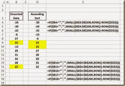
(Click On Image To See a Larger Version)
New or Changing Data
The advantage of sorting with formulas instead of the Data Sorting Tool is the formulas will automatically resort the data if any data is changed or additional data is added. The following changes were made to the data:-6 was changed to -7 (colored orange)
New data points 11, 13, and 14 were added (colored light blue)
The data is automatically resorted after these changes and additions. The Data Analysis Sorting Tool would have to be re-run manually to resort the data.

(Click On Image To See a Larger Version)
Multi-Column Sorting With the Data Sorting Tool in Excel
Multiple columns of data that require secondary or tertiary sorts require the use of the Data Sorting Tool. Alphabetic data can also be sorted using this tool. Below are 3 columns of data that will be sorted using a primary sort of Column 3, then a secondary sort of Column 2, and finally a tertiary sort of Column 1.
(Click On Image To See a Larger Version)
The first step is to highlight the data including the column headers if they are there as follows:

(Click On Image To See a Larger Version)
The Data Sorting Tool is found under the Data tab as follows:

(Click On Image To See a Larger Version)
Clicking on Sort brings up the following dialogue box. The column headers show up because they were highlighted with the original data in Step 1.

(Click On Image To See a Larger Version)
The following completed dialogue is set up to perform a primary sort of Column 3, then a secondary sort of Column 2, and finally a tertiary sort of Column 1.

(Click On Image To See a Larger Version)
Clicking OK performs that sort as follows:

(Click On Image To See a Larger Version)
No comments:
Post a Comment