This algorithm comes under the greedy method, which means that the objects are chosen to join a growing collection by iteratively picking an object that minimizes some cost function.
Now, taking account of the above mentioned greedy method, the Prim-Jarnik's algorithm is similar to the Dijkstra's shortest-path algorithm to grow the Minimum Spanning Tree (MST) from a single cluster starting with a randomly chosen single root vertex.
The Prim-Jarnik's algorithm can be broken down as follows:
Step 1: Define the starting "cloud" of vertices [C] by selecting some random vertex [v] initially
Step 2: Iteratively choose a min-weight edge [e=(v,u)], thereby connecting a vertex [v] in the cloud [C] to a vertex [u] outside of [C]. After choosing [e] the vertex [u] is brought into the cloud [C] continuously until a spanning tree emerges.
Pseudo-code of the Prim-Jarnik's algorithm
// Prim-Jarnik(G) [Time complexity = O(m * log * n)]
// Input: A weighted connected graph [G] with n number of vertices & m number of edges
// Output: A minimum spanning tree [T] for [G]
// Pick a root vertex [v] of [G]
D[v] <- 0
// All vertices connected to the root vertex, hence it necessary to define the cost function.
// The cost function "D[u] = +infinity" when vertex [u] doesn't connect to vertex [v].
for each vertex u != v do
D[u] <- +infinity
// Initialise the MST
T <- null
// Initialise a priority queue Q with an entry ((u,null),D[u]) for each vertex [u],
// where (u,null) is the element & D[u] in the key
while Q is not empty do
(u,e) <- Q.removeMin()
Add vertex u and edge e to T
// Perform the relaxation procedure on the edge of the vertex [z] adjacent to [u]
For each vertex z adjacent to u such that z is in Q do
if W((u,z)) <>
D[z] <- W((u,z))
Change to (z,(u,z)) the element of vertex z in Q
Change to D[z] the key of vertex z in Q
return the tree T


Kruskal's algorithm for extracting Minimum Spanning Tree (MST)
This algorithm comes under the greedy method, which means that the objects are chosen to join a growing collection by iteratively picking an object that minimizes some cost function.
Now, taking account of the above mentioned greedy method, the Kruskal's algorithm with a graph considers the edges in order of their weights to grow the Minimum Spanning Tree (MST) in clusters.
The Kruskal's algorithm can be broken down as follows:
Step 1: In a given undirected graph [G] consider each vertex is in its own cluster all by itself i.e. if a [G] has four vertices then you have four cluster initially
Step 2: Look for each edges in turn, ordered by increasing weight i.e. arrange all the edges in ascending order
Step 3: Start with the smallest weighing edge. If this edge connects two different clusters then it is considered as the min-weight "bridge" edge [e] and added to the set of edges of the MST. In this initial stages, due to addition of [e] to the MST (i.e. the growth of the MST), the two clusters then are merged into a single cluster. However, if a given [e] connects to two vertices that are already in the identified cluster then this [e] is discarded.
Step 4: Now iteratively the algorithm adds enough [e] to a set of edges of spanning tree, it terminates and outputs this tree as the MST.
Pseudo-code of the Kruskal's algorithm
// Kruskal(G) [Time complexity = O(m * log * n)]
// Input: A simple connected weight graph [G] with [n] vertices and [m] edges
// Output: A minimum spanning tree [T] for [G]
for each vertex [v] in [G] do
Define an elementary cluster C(v) <- {v}
// Initialise a priority queue Q to contain all edges in [G], using the weights as keys
T <- null
// The above [T] will ultimately contain the edges of the MST
while [T] has fewer then n-1 edges do
(u,v) <- Q.removeMin()
// Let C(v) be the cluster containing v, and let C(u) be the cluster containing u.
if C(v) != C(u) the
Add edges (v,u) to T
Merge C(v) & C(u)
// The above union of C(v) & C(u) yields a single cluster
return tree TExample below shows the Kruskal's algorithm that extracts the MST from a spanning tree. This spanning tree depicts a subset of Finnish intercity roadways route:
--------------------------------------------
Stage 1.
--------------------------------------------
Main cluster (C) contains the following vertices: null
Elementary Cluster (C1) contains the following vertices: null
Priority Queue (Q)
------------------
----
110
----
137
---
141
---
164
---
177
---
294
---
381
---
409
---
534
---
549
---
------------------
Set of min-weight "bridge" edges e = {null}
Set of discarded edges d = {null}
--------------------------------------------
Stage 2.
--------------------------------------------
Main cluster (C) contains the following vertices:null
Elementary Cluster (C1) contains the following vertices: Pori+Tampere
Priority Queue (Q)
------------------
----
137
---
141
---
164
---
177
---
294
---
381
---
409
---
534
---
549
---
------------------
Set of min-weight "bridge" edges e = {110}
Set of discarded edges d = {null}
--------------------------------------------
Stage 3.
--------------------------------------------
Main cluster (C) contains the following vertices:null
Elementary Cluster (C1) contains the following vertices: Pori+Tampere
Elementary Cluster (C2) contains the following vertices: Helsinki+Kouvola
Priority Queue (Q)
------------------
---
141
---
164
---
177
---
294
---
381
---
409
---
534
---
549
---
------------------
Set of min-weight "bridge" edges e = {110,137,}
Set of discarded edges d = {null}
--------------------------------------------
Stage 4.
--------------------------------------------
Main cluster (C) contains the following vertices:null
Elementary Cluster (C1) contains the following vertices: Pori+Tampere+Turku
Elementary Cluster (C2) contains the following vertices: Helsinki+Kouvola
Priority Queue (Q)
------------------
---
164
---
177
---
294
---
381
---
409
---
534
---
549
---
------------------
Set of min-weight "bridge" edges e = {110,137,141}
Set of discarded edges d = {null}
--------------------------------------------
Stage 5.
--------------------------------------------
Main cluster (C) contains the following vertices:null
Elementary Cluster (C1) contains the following vertices: Pori+Tampere+Turku+Helsinki+Kouvola
Priority Queue (Q)
------------------
---
177
---
294
---
381
---
409
---
534
---
549
---
------------------
Set of min-weight "bridge" edges e = {110,137,141,164,}
Set of discarded edges d = {null}
--------------------------------------------
Stage 6.
--------------------------------------------
Main cluster (C) contains the following vertices:null
Elementary Cluster (C1) contains the following vertices: Pori+Tampere+Turku+Helsinki+Kouvola
Priority Queue (Q)
------------------
---
294
---
381
---
409
---
534
---
549
---
------------------
Set of min-weight "bridge" edges e = {110,137,141,164,}
Set of discarded edges d = {177,}
--------------------------------------------
Stage 7.
--------------------------------------------
Main cluster (C) contains the following vertices:null
Elementary Cluster (C1) contains the following vertices: Pori+Tampere+Turku+Helsinki+Kouvola+Kuopio
Priority Queue (Q)
------------------
---
381
---
409
---
534
---
549
---
------------------
Set of min-weight "bridge" edges e = {110,137,141,164,294}
Set of discarded edges d = {177,}
--------------------------------------------
Stage 8.
--------------------------------------------
Main cluster (C) contains the following vertices:null
Elementary Cluster (C1) contains the following vertices: Pori+Tampere+Turku+Helsinki+Kouvola+Kuopio
Priority Queue (Q)
------------------
---
409
---
534
---
549
---
------------------
Set of min-weight "bridge" edges e = {110,137,141,164,294,}
Set of discarded edges d = {177,381}
--------------------------------------------
Stage 9.
--------------------------------------------
Main cluster (C) contains the following vertices:null
Elementary Cluster (C1) contains the following vertices: Pori+Tampere+Turku+Helsinki+Kouvola+Kuopio
Priority Queue (Q)
------------------
---
534
---
549
---
------------------
Set of min-weight "bridge" edges e = {110,137,141,164,294}
Set of discarded edges d = {177,381,409}
--------------------------------------------
Stage 10.
--------------------------------------------
Main cluster (C) contains the following vertices:null
Elementary Cluster (C1) contains the following vertices: Pori+Tampere+Turku+Helsinki+Kouvola+Kuopio+Oulu
Priority Queue (Q)
------------------
---
549
---
------------------
Set of min-weight "bridge" edges e = {110,137,141,164,294,534,}
Set of discarded edges d = {177,381,409}
--------------------------------------------
Stage 11.
--------------------------------------------
Main cluster (C) contains the following vertices = C1
Elementary Cluster (C1) contains the following vertices: Pori+Tampere+Turku+Helsinki+Kouvola+Kuopio+Oulu+Ivalo
Priority Queue (Q)
------------------
null
------------------
Set of min-weight "bridge" edges e = {110,137,141,164,294,534,549}
Set of discarded edges d = {177,381,409}


Spanning Tree & Minimum Spanning Tree (MST)
Spanning Tree - A tree that contains every vertex of a connected graph G is referred to as a spanning tree. The below figure depicts the Finnish intercity roadways route as a sapnning tree.

Minimum Spanning Tree (MST) - the problem of computing a spanning tree with the smallest total weight is known as the Minimum Spanning Tree problem. The below figure depicts the MST that houses a collection of smallest weighted routes between the Finnish cities. Routes not taken into the MST are: 177,381,409.


Minimum Spanning Tree (MST) - the problem of computing a spanning tree with the smallest total weight is known as the Minimum Spanning Tree problem. The below figure depicts the MST that houses a collection of smallest weighted routes between the Finnish cities. Routes not taken into the MST are: 177,381,409.

Friday, March 27, 2009
Application of a Binary Tree
The binary tree are applicable in the below mentioned fields:
- Used in the compilers of high-level programming languages for intermediate representation
- Used as a searching technique
- Used in databases for storing data
- To solve arithmetic expressions
- Used in the compilers of high-level programming languages for intermediate representation
- Used as a searching technique
- Used in databases for storing data
- To solve arithmetic expressions
Exercise-Binary Tree Construction
Given data items: 17, 6, 3, 9 ,12, 15, 1, 18, 22
The resulting binary tree is:
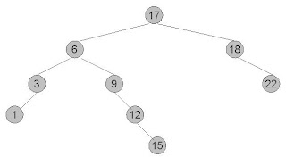
The resulting binary tree is:

What is a Binary Tree?
A binary tree embodies a finite set of data items that is either empty or partitioned into three disjoint subsets. The first part contains a single data item referred to as the root of the binary tree, other two data items are left and right subtrees. These data items is referred to as nodes of the binary tree.
 From this figure we can portray the following:
A - Root node of the binary tree
A - Parent node of the nodes B & C
B & C - Children nodes of A and these nodes are in a level one more than the root node A
C - Right child node of A
B - Left child node of A
D & E - These node are without a child, so they are referred to as leafs or external nodes
B & C - These nodes have a child each, so they are referred to as internal nodes
Depth of this binary tree - The longest path from the root node A to any leaf node, for example D node. Therefore, the depth of this binary tree is two.
Indegree of a node - The number of edges merging into a node. For example, indegree of the node B is one i.e. one edge merges.
Outdegree of a node - The number of edges coming out from a node. For example, outdegree of the node A is two i.e. two edges comes out of this root node.
Concerning the binary trees, do refer to the following blog entries:
- Exercise-Binary Tree Construction
- Application of a Binary Tree
What is a Complete Binary Tree?
A strictly binary tree of depth 'd' in which all the leaves are at level 'd' i.e. there is non empty left or right subtrees and leaves are populated at the same level.
In a complete binary tree all the internal nodes have equal degree, which means that one node at the root level, two nodes at level 2, four nodes at level 3, eight nodes at level 4, etc, which the below figure represents:
In a complete binary tree all the internal nodes have equal degree, which means that one node at the root level, two nodes at level 2, four nodes at level 3, eight nodes at level 4, etc, which the below figure represents:


